nlsLM擬合多條指數函數並繪製于ggplot
文章目錄
折騰了我兩天的
$$ y = c + (1 - a*e^{-bx}) $$
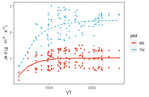
我估計會有人跟我一樣因爲數據不是很完善,nls擬合會出現singular gradient blabla的,這時候你需要一個更好的初始值,或者修改數據,但這都不是那麽好弄的,意外發現了一個nlsLM函數,試了下能用,但又發現好像不能夠直接像lm一樣同時畫兩條綫(最終效果見下圖)。soo,最終確定的思路是先做擬合,然後在ggplot2中畫出predict值
需要的包:
library(ggplot2)
library(ggsci) # 美化
library(dplyr) # 數據處理
library(minpack.lm) # nlsLM所在包
數據示例
      y      x        plot
1  0.2970262 493.735   PN
2  1.3179885 493.735   PN
3  1.7368123 493.735   PN
4  0.2275084 493.735   MT
5  0.2830588 493.735   MT
6  1.1175526 493.735   MT
指數擬合
首先我們要為這個數據框添加一列predict數據,然後根據x,y畫數據點;根據x,predict畫擬合綫
rbind(
  data %>%
    filter(plot == 'PN') %>% # 選出index為PN的數據進行擬合
    mutate(prd= # 這裏的初始值,沒有nls要求那麽嚴,多試幾次就行了,當然最好有大概範圍
             nlsLM(formula = Js.d ~ c+ a * (1 - exp( -b* VT )) ,
                   start = list( a= 0.1, b=0.0001, c=0.1)) %>% predict() ),

  data %>%
    filter( plot == 'MT') %>% # 選出index為MT的數據進行擬合
    mutate(prd=
             nlsLM(formula = Js.d ~ c+ a * (1 - exp( -b* VT )) ,
                   start = list( a= 0.1, b=0.0001, c=0.1)) %>% predict() )
)

# 得到擬合值
        y      x     plot    prd
1  0.2970262 493.735   PN 0.6158806
2  1.3179885 493.735   PN 0.6158806
3  1.7368123 493.735   PN 0.6158806
4  0.2275084 493.735   MT 0.6158806
5  0.2830588 493.735   MT 0.6158806
6  1.1175526 493.735   MT 0.6158806
擬合並作圖
(我並沒有儲存中間變量,所以直接用管道進行作圖,反正這個數據框用一次就不用的)
rbind(
  data %>%
    filter(plot == 'PN') %>%
    mutate(prd=
             nlsLM(formula = Js.d ~ c+ a * (1 - exp( -b* VT )) ,
                   start = list( a= 0.1, b=0.0001, c=0.1)) %>% predict() ),

  data %>%
    filter( plot == 'MT') %>%
    mutate(prd=
             nlsLM(formula = Js.d ~ c+ a * (1 - exp( -b* VT )) ,
                   start = list( a= 0.1, b=0.0001, c=0.1)) %>% predict() )
) %>%
  ggplot(aes( color = plot, shape = plot, linetype = plot))+
  geom_point( aes( x , y), size=1.5)+ #注意此處描點使用原數據
  geom_line( aes( x, prd),lwd=1.3)+   #而描綫使用擬合數據
  theme(panel.background = element_rect(fill = "white", colour = "grey10"))+ #去背景
  scale_color_npg()+  #美化
  labs(x= '' ,
       y= expression(paste(Js.d , ' (g',' · ', m^{-2}, ' · ', s^{-1}, ')')))
參數及P值
圖上不能直接顯示參數和P值,ggplot2在這方面有點弱,如果是綫性模型倒可以有ggpmisc包實現,但這個非綫性模型,我估計他沒這麽强,所以要手動提取
# 簡化版
data %>%
  filter(plot == 'MF') %>%
           nlsLM(formula = Js.d ~ c+ a * (1 - exp( -b* VT )) ,
                 start = list( a= .1, b=0.0001, c=0.1)) %>% summary %>%
  .[['parameters']] %>% .[,c(1,4)] %>% data.frame() %>%
    mutate(Estimate = round(Estimate,3 ),
           `Pr...t..`= round(`Pr...t..`, 3),
            para = c('a', 'b', 'c'),
            plot = 'MF')
做到這一步,就可以提取參數,P值,參數名,和index名了。
但這裏的代碼實際上是我的節選簡化版,我原始數據index中有index,可以理解爲大處理裏有小處理,上面一個圖是一個小處理,再加三個圖是三個大處理,所以我的提取參數代碼是這樣的
rbind(
  data %>%
  filter(Tree == 'Ss' & plot == 'TW') %>%
           nlsLM(formula = Js.d ~ c+ a * (1 - exp( -b* VT )) ,
                 start = list( a= .1, b=0.0001, c=0.1)) %>% summary %>%
  .[['parameters']] %>% .[,c(1,4)] %>% data.frame() %>%
    mutate(Estimate = round(Estimate,3 ), `Pr...t..`= round(`Pr...t..`, 3), para = c('a', 'b', 'c'), Tree = 'Ss' , plot = 'TW'),

  data %>%
    filter(Tree == 'Ss' & plot == 'MS') %>%
    nlsLM(formula = Js.d ~ c+ a * (1 - exp( -b* VT )) ,
          start = list( a= .1, b=0.0001, c=0.1)) %>% summary %>%
    .[['parameters']] %>% .[,c(1,4)] %>% data.frame() %>%
    mutate(Estimate = round(Estimate,3 ), `Pr...t..`= round(`Pr...t..`, 3), para = c('a', 'b', 'c'), Tree = 'Ss' , plot = 'MS'),

  data %>%
    filter(Tree == 'Cc' & plot == 'MT') %>%
    nlsLM(formula = Js.d ~ c+ a * (1 - exp( -b* VT )) ,
          start = list( a= .1, b=0.0001, c=0.1)) %>% summary %>%
    .[['parameters']] %>% .[,c(1,4)] %>% data.frame() %>%
    mutate(Estimate = round(Estimate,3 ), `Pr...t..`= round(`Pr...t..`, 3), para = c('a', 'b', 'c'), Tree = 'Cc' , plot = 'MT'),

  data %>%
    filter(Tree == 'Cc' & plot == 'MS') %>%
    nlsLM(formula = Js.d ~ c+ a * (1 - exp( -b* VT )) ,
          start = list( a= .1, b=0.0001, c=0.1)) %>% summary %>%
    .[['parameters']] %>% .[,c(1,4)] %>% data.frame() %>%
    mutate(Estimate = round(Estimate,3 ), `Pr...t..`= round(`Pr...t..`, 3), para = c('a', 'b', 'c'), Tree = 'Cc' , plot = 'MS'),

  data %>%
    filter(Tree == 'Pm' & plot == 'PN') %>%
    nlsLM(formula = Js.d ~ c+ a * (1 - exp( -b* VT )) ,
          start = list( a= .1, b=0.0001, c=0.1)) %>% summary %>%
    .[['parameters']] %>% .[,c(1,4)] %>% data.frame() %>%
    mutate(Estimate = round(Estimate,3 ), `Pr...t..`= round(`Pr...t..`, 3), para = c('a', 'b', 'c'), Tree = 'Pm' , plot = 'PN'),

  data %>%
    filter(Tree == 'Pm' & plot == 'PN') %>%
    nlsLM(formula = Js.d ~ c+ a * (1 - exp( -b* VT )) ,
          start = list( a= .1, b=0.0001, c=0.1)) %>% summary %>%
    .[['parameters']] %>% .[,c(1,4)] %>% data.frame() %>%
    mutate(Estimate = round(Estimate,3 ), `Pr...t..`= round(`Pr...t..`, 3), para = c('a', 'b', 'c'), Tree = 'Pm' , plot = 'PN'
) %>% rename(e = Estimate , p = 'Pr...t..') %>%  # 上面一串都是數據提取及合并

  xtabs(e  ~ para + plot+ Tree ,.) # swich first args to 'e' or 'p' to review

# 得到結果
, , Tree = Cc

    plot
para     MS     PN     TW
   a  1.667  0.000  3.564
   b  0.003  0.000  0.002
   c -0.638  0.000 -1.106

, , Tree = Pm

    plot
para     MS     PN     TW
   a  0.000  0.899  0.972
   b  0.000  0.001  0.001
   c  0.000  0.244  0.138

, , Tree = Ss

    plot
para     MS     PN     TW
   a  0.832  0.000  0.638
   b  0.003  0.000  0.001
   c -0.194  0.000  0.335
因爲我改過變量名,所以上面的代碼有錯漏,但這不重要,反正都是要調整的
加油~
- 原文作者:燈燈
- 原文鏈接:https://ferristale.com/draw-two-or-more-exponential-regression-simultaneously-with-nlsLM&ggplot2/
- 原文鏈接:本作品採用CC BY-NC-ND 4.0. 進行許可,非商業轉載請註明出處(作者,原文鏈接),商業轉載請聯繫作者獲得授權。